edge of chaos.

A Cellular Automaton (CA) is a spatially extended dynamical system represented by a lattice of cells where each cell is in one of several possible states. Often, the lattice is of one or two dimensions and each cell takes a value of “on” or “off”. At each time step the state of each cell is updated as a function of its neighbor’s states. The function used to update a cell is called a rule; there may be multiple such rules. One well known rule set is Conway’s Game of Life. This and many other rules can be explored using the cross-platform tool Golly.

Christopher Langton, a pioneer of Artificial Intelligence, studied one dimensional cellular automata in the early 90s. Langton examined why certain rules resulted in periodic, random, or highly structured behavior. He proposed that CA rules approaching a phase transition between ordered and disordered behavior are capable of universal (Turing complete) computation. There are several interpretations of what computation means in this context; perhaps the most straightforward views a rule as a program and the initial grid values (the initial configuration) as the program’s input.

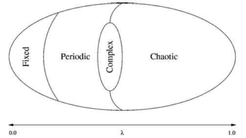
Langton described the computational capability of a CA using three properties: 1) memory, 2) transmission, and 3) information processing. The space of rules was studied using a parameter \(\lambda\) that gives the fraction of a CA’s rules resulting in an “on” state for a cell. He argued that diverging correlation times and lengths were necessary for memory and transmission, and these were maximized by values of \(\lambda\) between 0 (complete order) and 1 (complete disorder). For example, Conway’s Game of Life has \(\lambda = 0.273\) and is capable of universal computation given certain initial conditions. Other rules with different \(\lambda\) values may also permit universal computation. There is no standard value of \(\lambda\) that characterizes universal computation across all CAs, but values maximizing memory and transmission were found to exist near the “edge of chaos” between order and disorder. The validity of this claim is briefly discussed at the end of this tutorial.

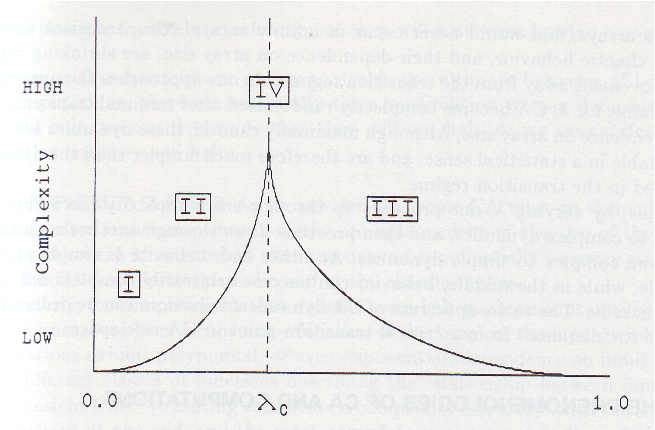
If you’ll forgive the resolution, the following figure from Langton’s Life at the Edge of Chaos illustrates these ideas using Wolfram’s universality classes:

The parameterization of rule-space using \(\lambda\) ties complexity to structure rather than randomness, and is similar to Crutchfield’s statistical complexity \(C_\mu\) and Grassberger’s effective measure complexity. A completely disordered (random) system can be described simply in probabilistic terms, as can a completely ordered system, but those systems in between exhibit more structured behavior and thus require more elaborate models. Crutchfield and Young made these ideas explicit in several papers including Inferring Statistical Complexity and Computation at the Onset of Chaos. This page serves as a tutorial for approximating the results from “Inferring Statistical Complexity” (henceforth ISC) using the Computational Mechanics in Python (CMPy) library.

reconstructing the route to chaos.

ISC demonstrates a \(\lambda\)-like phase transition in the period doubling behavior of the logistic map \(x_{n+1} = r x_n (1 - x_n)\). They observe this transition for progressively chaotic values of the parameter \(r\), generating a symbolic time series via the generating partition \({[0, 0.5), [0.5, 1]}\) and feeding this into the subtree merging \(\epsilon\)-machine reconstruction algorithm. From the \(\epsilon\)-machine, the entropy rate and statistical complexity of the underlying data stream is calculated and plotted.

It is recommended the reader is familiar with the above terminology before proceeding. The first figure we’ll reproduce is below:

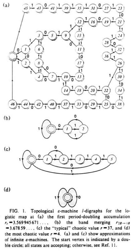
These \(\epsilon\)-machines are topologically reconstructed: morphs (subtrees) are equivalent if branch symbols match regardless of the associated probability.

Our first task is obtaining data from the logistic map and applying the generating partition:

def logistic_generate(r, data_length=100000):
    data = range(data_length)
    x = numpy.random.random()

    # skip transients
    for i in xrange(10000):
        x = r * x * (1 - x)

    for i in xrange(data_length):
        data[i] = 0 if x < 0.5 else 1
        x = r * x * (1 - x)

    return data

Next we infer machines for the given \(r\) values:

for morph_length, r in zip([16, 6, 6, 6], [3.569945671, 3.67859, 3.7, 4]):
    print r
    m = Merger(logistic_generate(r), morph_length)
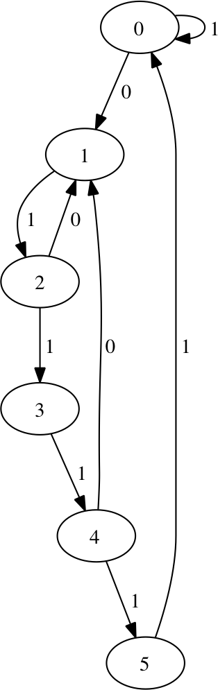
    m.write('r%.2f.dot' % r)

The resulting machine for \(r=3.569945671\) is here due to size. Note that states 47 and 48 transition back to the start state on any symbol, denoted with transition symbol \(*\). For \(r=3.67859\) we have:

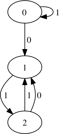
and for \(r=3.7\):

and finally for \(r=4.0\):

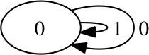
This single-state machine captures the total lack of causal structure in the chaotic regime of the logistic map.

the complexity-entropy diagram.

The next figure plots an estimate of the entropy rate against the statistical complexity of the inferred \(\epsilon\)-machine for 193 realizations of the logistic map’s generating partition, using progressively chaotic \(r\) values:

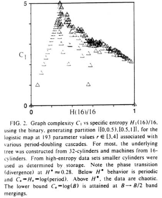
Entropy rate is estimated using length-\(L\) blocks:

\[ h_\mu(L) = \frac{H(L)}{L} \]

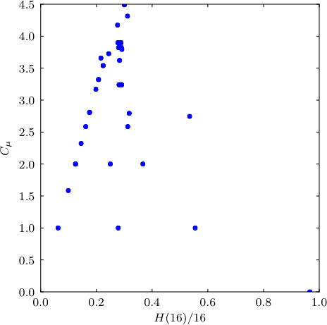
The plot is relatively straightforward: we generate a list of \(r\) values, generate partitioned data, infer the \(\epsilon\)-machine, and store the entropy estimate and statistical complexity. To create the diagram, we pass these values to matplotlib’s plot function.

rs = numpy.linspace(3, 4, 193)
morph_length = 6
h_mus = []
c_mus = []

for r in rs:
    data = logistic_generate(r)
    m = Merger(data, morph_length)

    h_mus.append(entropy(data, block_length=16) / 16.0)
    c_mus.append(statistical_complexity(m))

pylab.plot(h_mus, c_mus, '.')
pylab.ylabel('$C_\mu$')
pylab.show()

This approximates the figure from ISC since we have different data and parameter values, but the overall structure should be similar — complexity grows towards the cited peak at \(H^* \approx 0.28\) followed by a gradual decrease as \(r\) moves toward complete chaos:

This conceptually maps back to Langton’s plot of \(\lambda\) versus complexity for Wolfram’s CA universality classes:

In their paper Revisiting the Edge of Chaos, Mitchell, Hraber, and Crutchfield challenge the CA interpretation of the edge of chaos. They show that rules performing complex computation need not be near \(\lambda_c\) and argue for more rigorous definitions of computational capability, complex computation, and the edge of chaos itself. Shalizi gives a further critique of the historical misappropriation of the edge of chaos label.